why staying in touch is brutal (statistically)
preface
Every year, millions of incoming first-years leave their hometowns behind. Recently, Instagram or even LinkedIn has made it easier (and more annoying) to hear about and speak with people you don’t meet everyday. But do we really stay in touch?
Before we begin, much of what you’re about to read will make me sound like (a) a mad scientist (b) someone who does not know to make friends or (c) both. Statistically analysing how a friendship fades is pretty dystopian, but loads of (really smart) people have made careers out of studying how people interact, form relationships and grow.
TL;DR - this is math, not social advice.
formalizing a statistical “friendship”
With that cheerful introduction out of the way, we can start with some axioms.
TL;DR - Everyone you meet gets a number for how close you are, not talking depletes friendships, talking = interactions, and interactions are random.
Every friendship can be ascribed a continuous time-varying degree of closeness. As time passes, we get closer to some people but further from others. This “closeness” is quantifiable.
isn't that weird?
At first glance, this seems weird. We aren’t in the habit of constantly evaluating everyone based on how close we are. Or are we?
Every time we get conflicting social schedules, we subconsciously pick a particular person or group to hang out with. Say you’re offered dinner with A or games night with B on the same night, you must pick one. And we do this every single day, whether it’s plans, conversations, car rides, messages etc. Going deeper, we’re all an individual repository of what’s called ranked choice voting (super common technique in some US jurisdictions) which basically means we subconsciously create tier lists of everybody we know based on choices. These tier lists could hypothetically be assigned values of closeness.
Ignored friendships decay over time. The less we interact with people, the weaker or ‘less close’ our friendships become. We can assume that there is uniform decay (such that the amount by which closeness decreases can be modelled mathematically) but more on that in a minute.
Every individual friendship has a series of “interactions”. Every time we text, call or meet someone, we can log that as an interaction. The simplest way for us to deal with this is to bump up closeness to its maximum value everytime we interact with someone.
why?
The math here can be a little hand-wavy, but socially, it makes sense – meeting people makes you closer to them again.
Still, this is sketchy, at best. Texting someone a half-hearted ‘Happy Birthday!’ probably doesn’t get you back to best friends immediately, but it’s helpful to ignore these as suboptimal interactions. Any interaction we log, then, has to be meaningful.
Interactions are a random occurrence. Outside of environments like class or social groups, interactions can be considered random. We can formalise this by setting an average rate of interactions $\lambda$ over a time period. If you meet C only when D hosts a party a couple times a year, then $\lambda \approx 2$ interactions per year.
explain?
Whether you run into them on the street, at the supermarket or at a party, interactions with acquaintances are pretty random, both in the mathematical and social sense.
The more statistical reader has probably gauged that this is leading up to a Poisson distribution, but in general, we tend to subconsciously talk about this anyway. When we say “I see her every spring” or “We meet whenever I go to New York”, we basically express averages in natural language form.
Okay, now for the math.
groundwork
Let’s try to quantify some of our basics. Rather than ranking everybody, let’s just say each individual friendship has a maximum degree of closeness $F_{max}=1$. Every meaningful interaction bumps our closeness back to $F_{max}$. In general, closeness $F ≥0$.
But how does closeness vary? Well, it’s reasonable to assume that the variation of closeness is related to the current closeness (when you’re good friends, not talking for a bit might change things; when you barely talk, continuing the silence hardly matters). Mathematically,
$$ \frac{dF}{dt}=-kF $$This is a trivial differential equation, and it can be solved using variable separation.
$$ \int\frac{1}{F}dF = \int-kdt $$$$ F = F_0e^{-kt} $$The use of $F_0$ comes from plugging in $t=0$ with the final constant. Also, as you might have already noticed, this form of modelling is really similar to radioactive decay in physics. Before we go ahead, it’s worth reflecting on what exactly $k$ is. To start with, we can quantify the initial closeness of a friendship by setting $F_0=10$ and investigate some graphs.
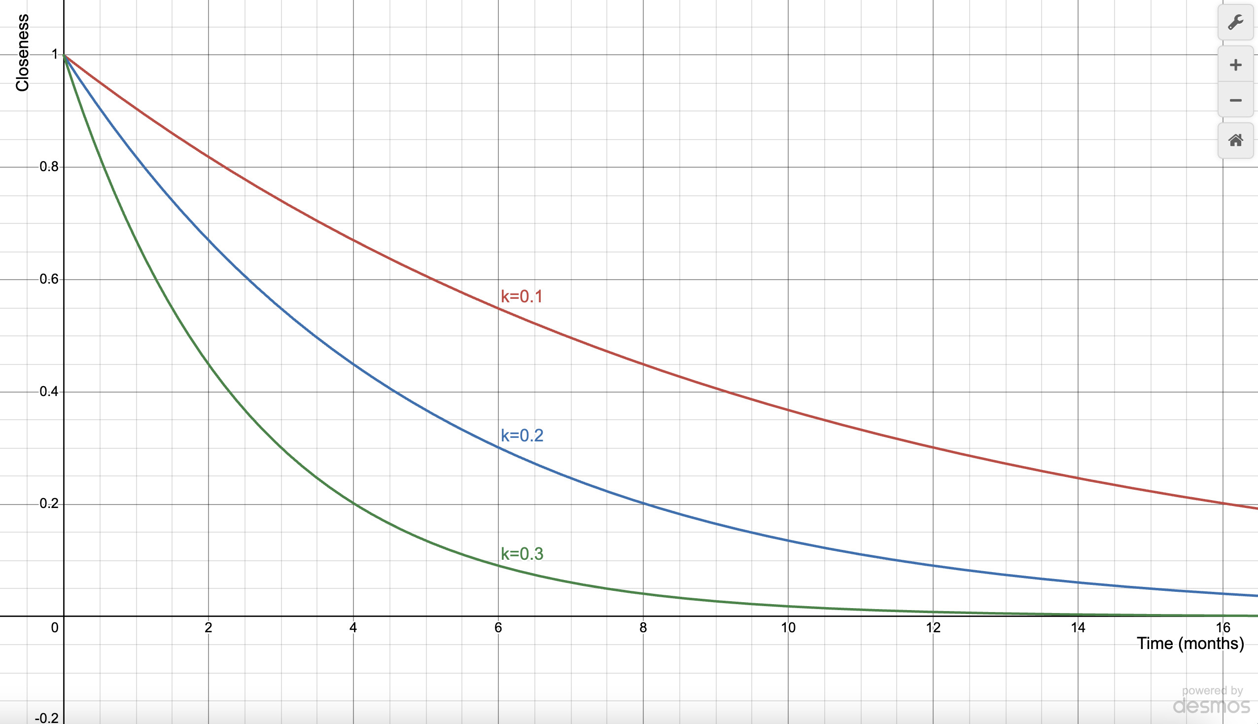
It appears, at least from the graphs’ behavior, that $k$ refers to how much effort a friendship needs. For lower values of $k$, the friendship requires less effort to maintain since closeness declines slower. We could have reached the same conclusion through derivatives, but the graphical interpretation makes it a little more obvious. So, we could call $k$ our maintenance constant, and assign values based on how high-maintenance a friendship is. If this seems extremely restrictive, we could, in theory, have any number of categories. (The units of $k$ here would be $\frac{1}{months}$ but I’ve omitted that for readability)
| Friendships | k-values |
|---|---|
| High-Maintenance | k=0.3 |
| Mid-Maintenance | k=0.2 |
| Low-Maintenance | k=0.1 |
Still, this is very strange - if people were easy to put into categories, this article would be pointless. Let’s try to work backwards. From the closeness equation, we can calculate the half-life of a friendship (by setting $F=0.5F_0$).
$$ t_{\frac{1}{2}}=\frac{\ln(2)}{k} $$This is actually great for a couple of reasons.
- It doesn’t make sense to wait till “closeness” hits zero since this never actually happens (exponential decay is asymptotic to the x-axis). BUT it does help to pick the half-life as a minimum friendship threshold. Basically, friendships are lost (or atleast in a bad spot) once you’re half as close as you were originally
- Defining friendships via half-lives is quite the improvement on our allocation of arbitrary values to $k$ based on graphs. For example, let’s say you consider not interacting for 3 months to be the threshold beyond which a friendship isn’t the same. This means $k=\frac{\ln(2)}{3}\approx0.23105$. If we ever do need to adjust for low or high maintenance friendships, it becomes much easier to do so via half-lives.
sanity check pt1
That was a lot of yapping. To cut through the bunch of assumptions and explanations, let’s actually run some calculations.
For our category model,
| k | half-life (months) |
|---|---|
| 0.1 | 6.931 |
| 0.2 | 3.466 |
| 0.3 | 2.310 |
For our half-life model,
| half-life (months) | k |
|---|---|
| 3 | 0.23105 |
| 6 | 0.11552 |
| 12 | 0.05776 |
But, thankfully, we do actually talk to people. So how do we study those interactions?
quantifying interactions
To quantify these interactions, we want to use something called a Poisson distribution, which requires the events to be random, independent, and occurring at some average rate $\lambda$. Most of us randomly reach out to people only when we remember them, so we can assume they follow a Poisson distribution.
$$ P(X=x) = \frac{(\lambda t)^xe^{-(\lambda t)}}{x!} $$The probability of meeting someone $x$ times in a given interval $t$ (let’s say a month) can be expressed in terms of the average rate of interactions in that interval $\lambda$, and Euler’s number $e$.
Stepping back for a second, we now have two competing forces.
- The exponential decay of closeness (you talk less and less)
- The Poisson-distributed ‘bumps’ or interactions (talking = reset to full closeness)
Basically, after every ‘bump’, closeness decays exponentially until the next bump. Visually,
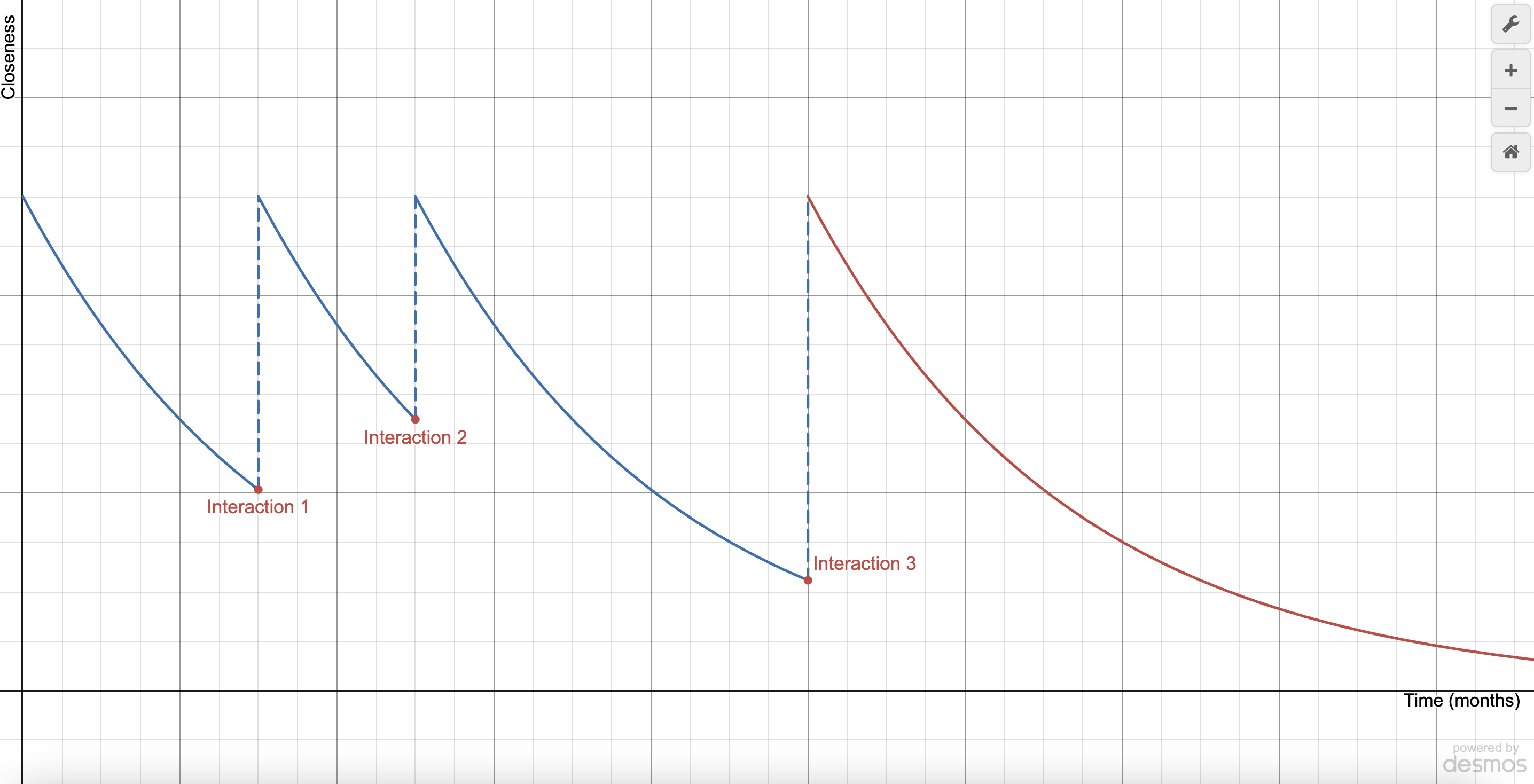
After the 3rd interaction, no interactions took place, and the friendship faded. The occurrence of interactions is governed by the Poisson distribution, while the behavior of the graph between interactions is governed by the exponential decay model.
You’ve probaby noticed that this graph ignores the cutoff of the half-life model , especially before the 1st and 3rd interactions, but we’re keeping that separate for the moment, just to get a feel for how a typical closeness pattern might look. In a second, we’ll add it back for the full picture.
sanity check pt2
We’ve made a bunch of assumptions and a cool graph but what does this mean in a practical sense? Let’s try it with a real person, say someone you meet three times a year on average at a party hosted by a mutual friend. In one year, $\lambda=0.25$ interactions per month.
Over a 12-month period, the probability of having 0 interactions can be expressed as
$$ P(X=0)=\frac{(\lambda t)^xe^{-\lambda t}}{x!}=e^{-\lambda t} $$$$ P(X=0)=e^{-3}\approx0.04979 $$Thus, there’s only a ~5% chance of losing this friendship in a year.
However, if you only meet once a year on average, then $\lambda=\frac{1}{12}$ interactions per month. Over a 12-month period, the probability of having 0 interactions can be expressed as
$$ P(X=0)=e^{-1}\approx0.36788 $$So, now, that’s nearly a 40% chance of losing this friendship in any given year.
reconciling decay with interactions
Now that we have a good model for interaction frequency and how closeness decays between interactions, we can combine both. In essence, what are the odds that two people interact before the friendship is lost? This is actually easier than it seems.
We require atleast one interaction over a given half-life $t_{\frac{1}{2}}$.
$$ P(X\ge1)=1-P(X=0)=1-e^{-\lambda t} $$We could try calculating this for a bunch of different half-lives and interaction frequencies, but it’s quite a bit more interesting (and visually appealing) to plot a map.
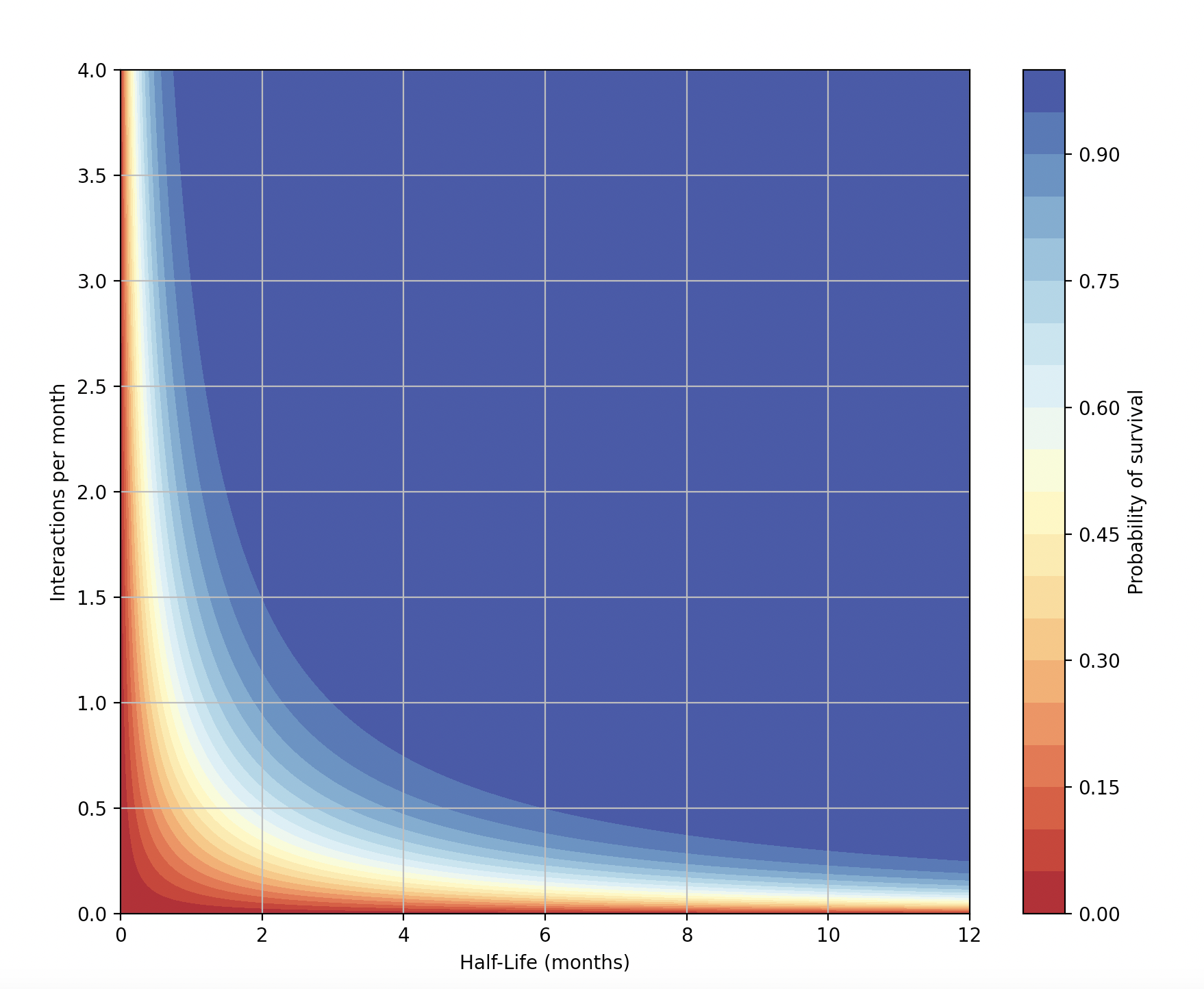
This looks interesting! That massive blue region indicates friendships that are basically guaranteed to survive. And we’re really only starting to see risks with high-maintenance friendships (half-life < 2 months) that have reasonably low interactions (< 1.5 per month).
So, maintaining connections seems to be easier than ever. But is it?
monte carlo
Maintaining one friendship seems to be pretty easy (as it should be). But what if we tested this empirically? Monte Carlo simulations let us run the same situation many times (in this case, we’re going with 10,000 trials) and see if our theoretical conditions hold up under the influence of random variables.
Let’s start with high-maintenance friendships. We can set $\lambda=0.25$ interactions per month (once in 4 months) and take our half-life of 3 months. There is a disparity here, but it can’t be that bad, right?
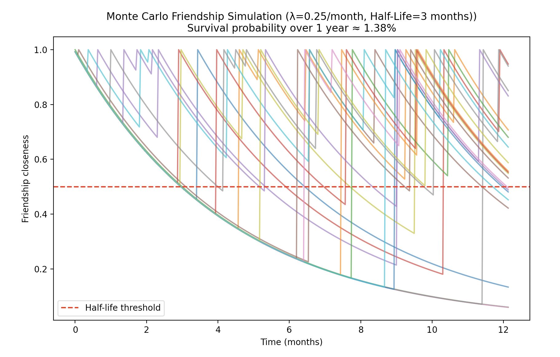
Wrong. The reason this survival probability is so bad has to do with fundamental probabilities. In a very hand-wavy sense, your friendship has to get through four 3-month periods in a year, and it can never dip below 0.5. More specifically, the odds of interaction in one 3-month period are only
$$ 1-e^{-0.25\times3}=0.52763=52.763\% $$Pretty bad.
Okay, but if we set $\lambda=0.25$ interactions per month and assume a half-life of 4 months, you’d expect that we’d have reasonably good, if not great chances of keeping the friendships.
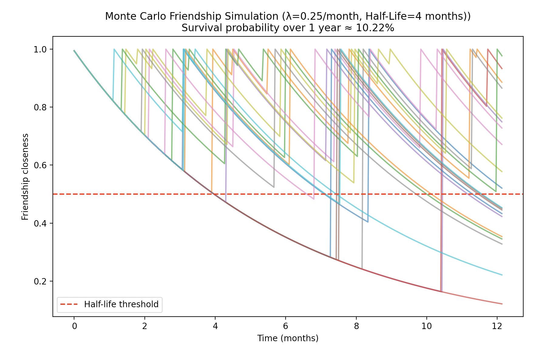
That’s… kinda underwhelming. Over one year, only 1 in 10 of these friendships will survive, even though the half-life and interaction frequency seem to line up. Mathematically, though, this actually makes sense. For any given friendship, the odds of an interaction in a 4-month period are
$$ 1-e^{-0.25\cdot4}=0.63212=63.212\% $$Good, but not great.
What if we consider mid-maintenance friendships, with 6-month half-lives?

This looks much more promising! We’ve effectively quadrupled the survival probability. Still, in a practical sense, this means losing half your friends every year, which is probably not ideal. What about low-maintenance?
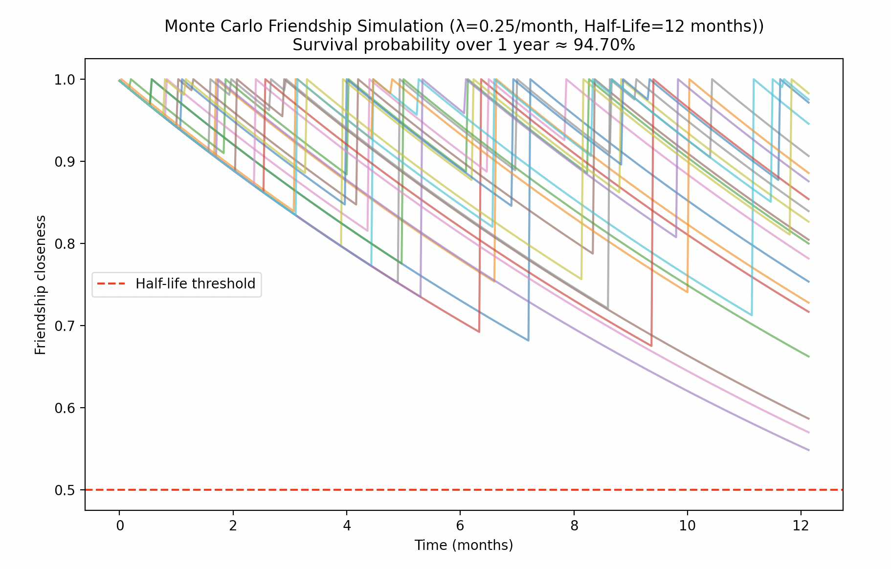
Immediately incredible. And again, this ties back to the original Poisson calculation.
limitations
This is a reasonably accurate, if rudimentary model. It does bring up a few limitations, stuff that I hope to address and refine in the future.
- $\lambda$ is constant, when in reality, interactions aren’t totally independent. The more we meet people, the more or less frequently we interact after.
- Interactions aren’t necessarily positive.
- Interactions need not bump up closeness to its maximum, and often only partially restore it.
conclusion (sanity check pt3)
So, is staying in touch brutal? Well, it depends.
A lot of the math above suggests that low-maintenance friendships are great. But in reality, people aren’t so easy to shoehorn into “maintenance” categories. We meet loads of amazing people, and it’s awfully reductionist to discard friendships purely based on how likely you are to stay in touch. At the risk of sounding too poetic, it might be better to enjoy the half-life than maximise its potential.
You also might have noticed the assumption of $\lambda=0.25$ interactions per month throughout our Monte Carlo simulations. This might seem too stringent - after all, we talk to people more than 3 times a year. But I’m going to end by reminding you of what an ‘interaction’ is, and how it must make a meaningful addition to your ‘closeness’. Still, it might be worth questioning - would a series of small mini-interactions have the same net effect as a meaningful interaction? And the answer - probably. So reach out to that person before the half-life ends!
But then again, this is math, not social advice.